Finalizer
Analyzer
Spectral Dynamic Contour (SDC)
The Spectral Dynamic Contour gives an overview of the full track, both spectrally and dynamically. This is a brand-new and highly useful approach to metering for mastering and the amount of visual feedback is comprehensive. While your ears are the most important instrument, relevant visual feedback will support what you hear and help you in choosing precise and fast solutions.
The SDC will help you identify how a processing change, intended for fixing a local issue, will affect the whole audio file. It will show how a dynamic process may affect lower levels than expected due to settings of attack and release times. And you will get useful insight when comparing against related album tracks and genre-specific reference tracks.
Six contour curves are represented, as shown below.

Key
The SDC curves show the level at each frequency as follows:
1. The maximum signal level at each frequency. This typically occurs a small amount of time in the track
4. The level at each frequency is below this line 50% of the time in the track (median). This is the ‘typical’ level of that frequency
6. The softest signal level in the track, at each frequency.
The six SDC contour curves together show the spectrum and the dynamics of the full track, both of which are essential when mastering music.
The X-axis is the frequency, corresponding to the frequency bands each 1/6th octave wide, that the SDC is based on. The Y axis shows the levels of the energy distribution in each frequency band. At a given frequency, the higher the SDC curves, the more energy is in that band. The closer together the curves are, the less dynamic the content is, in that band.
The SDC curves are affected by the Loudness Compensation in the Monitor section. For example, if the Loudness Compensation turns the level down, the SDC curves are also lowered accordingly. “What you hear is what you see.”
Examples of SDC
The following shows some examples of using the SDC with A, B, and REF.
SDC in A Mode (prepared source track)

In this example, the prepared source file is displayed, showing the spectral and dynamic content and its six contour curves. No effects (modules) are shown, as this is the pre-processed “before” source file. This includes the initial Level Normalization and Sample Rate Conversion, if applied (both located in the Prepare module). Note that the curves have the same colour as the “A” button, and the top curve is brighter.
SDC in B Mode (processed track)
1. No processing modules except the Limiter

In this example above, the processed output is shown, but no processing modules have been inserted yet, only the final Limiter module is in the chain. Note that the curves have the same colour as the “B” button, and the top curve is brighter.
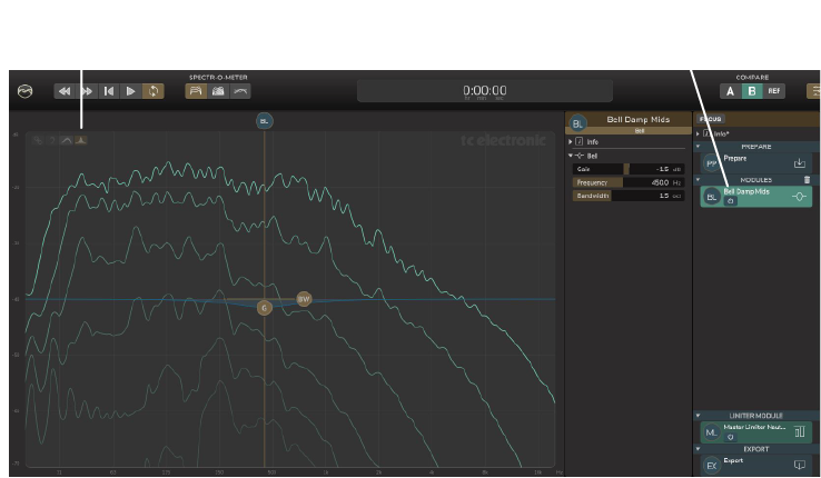
2. SDC in B mode, example with one processing module included

In this example, the “Bell Damp Mids” EQ module was inserted into the Module List, and note that the processed output has a slight dip in levels at the frequency of the filter, compared to the previous picture.
3. SDC in B mode, Difference Toggle
To avoid having to switch between the prepared source signals (A mode) and the processed signals (B mode), to see the difference between them, select the Difference button in the top left corner of the graph as shown. Select it again to turn the difference display off, and just show the B mode curves again. Note that the Difference button is only selectable from the B mode display (as B represents the processed track).
Note that the difference between A and B is also affected by the setting of the Loudness button in the Monitor section in order to “see what you hear”.

The Loudness Compensation will align A and B in loudness. This is great for hearing fine spectral and dynamic differences, and at the same time it also makes the SDC Difference highlight the processing performed while ignoring the overall loudness difference between A and B. Typically the Loudness Compensate yields a smaller and more relevant difference between A and B – both when comparing by listening and via the SDC.
4. Tips for working with the SDC
- Closely-spaced curves indicate low dynamics in that specific frequency/level range. This may be due to a dominating instrument having little dynamics due to the sound structure, or due to a well-rehearsed and consistent playing style, or it may be due to significant dynamics compression.
- The upper SDC curves can show content that “stick out” of the mix. It may be useful to examine if this is intentional, or if it could need a bit of help, for example by using the Dynamic EQ.
- The SDC Difference will show the combined effect of the processing modules in the chain. This is based on a time/frequency-analysis of the entire track, so it is great to give an overview of the processing performed, and how it affects the track.
- Selecting a Region will trigger a new SDC that applies only to that region. This is useful for ‘zooming in’ on a certain passage in the track, and investigating its spectral and dynamic properties.
5. EQ Curve Overlay Toggle
The EQ curve corresponding to the EQ modules (not the dynamic modules) can be shown as an overlay on top of the SDC. To always see the EQ curve overlaid on the graph, select the button in the top left corner of the graph as shown. Select the button again to turn the overlay off. This button is not available in REF mode, or if the selected Module does not feature an overlay.

When the EQ overlay is on, the EQ curve will be displayed and remain, as shown in the example below. Note: If this EQ overlay is off, the EQ curve will be shown momentarily if the mouse is moved close to the EQ controls (BL, G, and BW in this example).
In the example below, the Difference button is on, and so is the EQ overlay. The thicker filled areas show exactly the spectral and dynamic changes between the prepared source A and processed B, caused by the application of the Bell Damp Mids module. All SDC curves are affected equally, as the EQ will affect all signal levels (as opposed to a dynamic module).