Finalizer
Analyzer
Real Time Spectrum (RTS)
The RTS is a highly detailed version of well-known and popular spectrum analyzers, and shows a real-time spectrum behind the full track Spectral Dynamic Contours (SDC), described in the previous section. The RTS features shows two curves: a real-time peak analysis, and a moving-average real-time RMS analysis shown in the lower filled curve.
In addition to being an important and useful tool, by supporting your ears and decisions in the mastering process, the RTS can also complement the SDC curves: the RTS shows the relation between what you are hearing and the properties of the full track. Thereby you can determine exactly what instruments and passages in the track correspond to which peaks in the contour lines of the SDC
You will for example, see that the RTS Peak curve over the time of your track will “describe” the SDC top curve, while the lower RTS curve will often tend to move around the 3rd to 5th SDC curve.

Key
- The upper filled curve is a real-time peak analysis
- The lower filled curve is a moving-average real-time RMS analysis
The peak level analysis of the RTS is also based on an RMS level analysis and should not be confused with the True-Peak level of the Main Meter section.
The RTS will show which parts of the current content (at the playhead location) correspond to a specific part of the full track Spectral Dynamic Contours.
Note that if the track is not playing, then only the SDC curves will be displayed.
The RTS (and SDC) curves are affected by the Loudness Compensation in the Monitor section. For example, if the Loudness Compensation turns the level down, the RTS (and SDC) curves are also lowered accordingly. “What you hear is what you see.”
Examples of RTS
The following shows some examples of using the RTS.
RTS in A Mode (prepared source track)
In the example above, the prepared source A is displayed, with the top filled-curve showing the real-time peak analysis, and the lower filled-curve showing a moving-average real-time RMS analysis. These two moving curves are overlaid on the SDC spectral and dynamic content and its six contour curves. No EQ effects are shown, as this example is the prepared source file. Note that the two filled RTS curves have the same colour as the “A” button, and as this is happening in real time, the RTS curves are only shown when the track is playing.
RTS in B Mode (processed track)
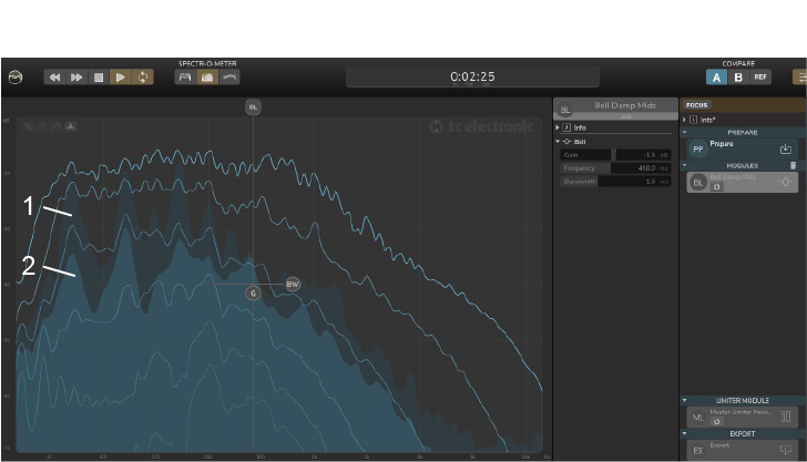
1. RTS in B mode, example with one optional processing module included.
In the example above, the Bell Damp Mids EQ module was included in the Modules List, and the processed output shows a dip in levels at the frequency of the filter. Note that the two filled curves and SDC curves have the same colour as the “B” button.
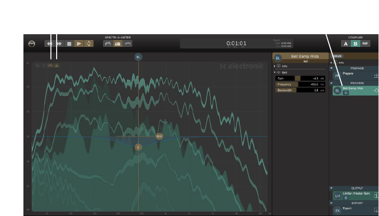
2. RTS in B mode, Difference ON
The Difference button affects the six SDC curves, as described previously for the SDC, and does not affect the two RTS filled curves. It is used to view the difference between source track (A mode) and the processed track (B mode). Select it again to turn the difference display off. Note that the Difference button is only selectable from the B mode display.


In the example above, the Difference button is on, and so is the EQ overlay. The two filled curves of the RTS and the SDC curves are affected by the controls of Bell Damp Mids EQ module. The filled areas of the SDC curves show exactly the spectral and dynamic changes between the source A and processed B, caused by the application of the Bell Damp Mids EQ module. If the display gets too “busy” to visualize clearly, it may help to turn off the EQ overlay once the EQ controls are set, and turn off the Difference toggle in the RTS view.